Amino acids
Isoelectric point & amino acids
In general, the isoelectric point, or pI, represents the pH value at which a molecule acquires a net zero charge under an electric field, that is, its positive charges cancel each other out with the negative charges. It is usually obtained experimentally by kinetic measurements, such as Zeta potential, electrofocusing or capillary electrophoresis. Similarly, the isoionic point refers to the same condition, however in the absence of an electric field, and can be measured by potentiometric titration, viscosity, or by the structural information of a monomeric sequence, such as in the primary sequence of proteins.
Since all 20 amino acids that make up the protein structure have ionizable groups, both in their carbon skeleton and in their side chain, it is possible to predict the isoionic point of an amino acid based on the pKa values presented in these ionizable groups. The pI is also commonly called the isoelectric point, although this definition entails a more complex theoretical scope.
Since all 20 amino acids that make up the protein structure have ionizable groups, both in their carbon skeleton and in their side chain, it is possible to predict the isoionic point of an amino acid based on the pKa values presented in these ionizable groups. The pI is also commonly called the isoelectric point, although this definition entails a more complex theoretical scope.
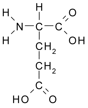
For example, glutamic acid (Glu, E) has an ionizable carboxylate in its side chain, in addition to the amine (-H\(_2\)N) and carboxylate groups of the carbon skeleton Figure 1:
Thus, its net net charge, qnet, can be determined from the sum of the acidic (qa) and basic (qb) forms of the molecule, in a similar way as that presented from the equation \(\eqref{eq-HHfosf}\):
\[ qnet = qb + qa \tag{1}\]
\[ qnet = qb+\frac{1}{1+10^{pH-pKa}} \tag{2}\]
Since this is a polyprotic acid, Equation 2 becomes:
\[ qnet = \sum_{i=1}^{n} {(qb+\frac{1}{1+10^{pH-pKi}})} \tag{3}\]
, with pKi as the nth value of pKa. In this way, it is possible to programmatically determine the titration curve of glutamic acid as a function of its charge, and not of the acid fraction. In this line, qb represents the form of the compound in base, which for Glu will present the values of -1 for the two carboxylates, and 0 for the amine group, making it necessary to compose an additional vector for qb.
# Glu Titration

qNet <- function(pH, qB, pKa) {
x <- 0
for (i in 1:length(qB)) {
x <- x + qB[i] + 1 / (1 + 10^(pH - pKa[i]))
}
return(x)
}
qB <- c(-1, 0, -1)
pKa <- c(2.2, 9.7, 4.3)

curve(qNet(x, qB, pKa), 1, 12, xlab = "pH", ylab = "qNet")

abline(0, 0, lty = "dotted")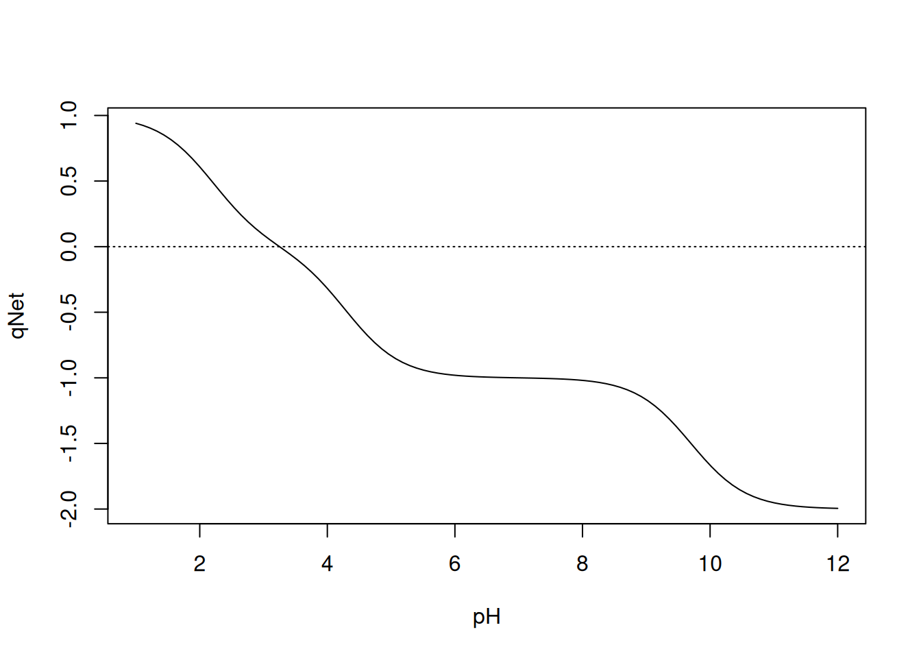
It is possible to manually identify the pI value for glutamic acid using an R function, such as
locator() seen previously. But it is also possible to access this value automatically, by applying a command that finds the root of this function, that is, the pH value that corresponds to a null value for qnet. For this, the use of uniroot is exemplified, in which the desired mathematical function is defined, as well as the lower and upper limits for the search by the algorithm, as follows:# Calculation of pI
f <- function(pH) {
qNet(pH, qB, pKa)
}
str(uniroot(f, c(2, 5)))List of 5
$ root : num 3.25
$ f.root : num -4.8e-06
$ iter : int 4
$ init.it : int NA
$ estim.prec: num 6.1e-05This result translates to a pI of 3.25 (
This way of obtaining a value using numerical calculation is sometimes called a numerical solution. On the other hand, the pI value for Glu can be obtained by a simpler procedure, usually found in textbooks on the subject, and which takes the form below:
root), in 4 iterations, with an estimated precision of 6.1x10\(^{-5}\), and an associated error of -4.8x10\(^{-6}\).This way of obtaining a value using numerical calculation is sometimes called a numerical solution. On the other hand, the pI value for Glu can be obtained by a simpler procedure, usually found in textbooks on the subject, and which takes the form below:
\[ pI = \frac{pKa1+pKa2}{2} \tag{4}\]
In our example, the pI will involve the pKas of the two carboxylates, which will result in (2.3+4.2)/2, or 3.25! Not bad for an approximation, huh? This procedure involving the solution of a mathematical problem based on system parameters is called an analytical method or solution. This solution can also be exemplified by the parameter obtained based on the observation of the graphical behavior of the titration, as in the figures above.
Now, what use is a more complex numerical procedure if a simple analytical equation already solves the problem of finding the pI value for glutamic acid? Well, exactly for that, to solve more complex problems. A little less rhetorically, however, it can be said that the numerical solution works better for systems where the analytical solution is sometimes not enough or even becomes impossible, as in the solution of equations with dozens of parameters.
Isoionic point & biopolymers
A situation on this topic can be illustrated by obtaining the pI value for a protein. For example, human lysozyme , an enzyme with a tertiary structure composed of 130 amino acid residues. In this case, the analytical solution is faced with the complexity of identifying which of these residues are ionizable in aqueous solution, and which would be involved in a distribution that would result in a net zero charge for the molecule.
For this more complex system, it is necessary to slightly expand the function defined for glutamic acid, computing in the qb vector the base charges of the 7 amino acids with ionizable side chains, and assigning a new vector for the quantity of each ionizable residue present in lysozyme. The code below exemplifies this solution, calculates the pI of the enzyme, and plots the graph of its titration, although this order is not relevant, since the pI is calculated numerically, not graphically.
# Lysozyme Titration and pI Determination

# Define function for qNet
qNet <- function(pH, qB, pKa, n) {
x <- 0
for (i in 1:length(qB)) {
x <- x + n[i] * qB[i] + n[i] / (1 + 10^(pH - pKa[i]))
}
return(x)
}

# Define pKas of aCOOH, aNH3 and the 7 side chains of AA
pKa <- c(2.2, 9.6, 3.9, 4.1, 6.0, 8.5, 10.1, 10.8, 12.5)

# Define qB, the charges of each amino acid in the base form
qB <- c(-1, 0, -1, -1, 0, -1, -1, 0, 0)

ionizable <- c(
"aCOOH", "aNH3", "Asp", "Glu", "His", "Cys", "Tyr",
"Lys", "Arg"
)
n <- c(1, 1, 7, 3, 1, 8, 6, 5, 14) # List of amounts of residues
# ionizable in lysozyme (each element represents the amount
# of aCOOH, aNH3, and certain AA in the enzyme)

# Calculation of pI
f <- function(pH) {
qNet(pH, qB, pKa, n)
}
str(uniroot(f, c(1, 13))) # estimation of pI between 10 and 12
List of 5
$ root : num 9.46
$ f.root : num 3.3e-07
$ iter : int 7
$ init.it : int NA
$ estim.prec: num 6.1e-05# Titration graph
curve(qNet(x, qB, pKa, n), 1, 12, xlab = "pH", ylab = "qNet")
abline(0, 0, lty = 3)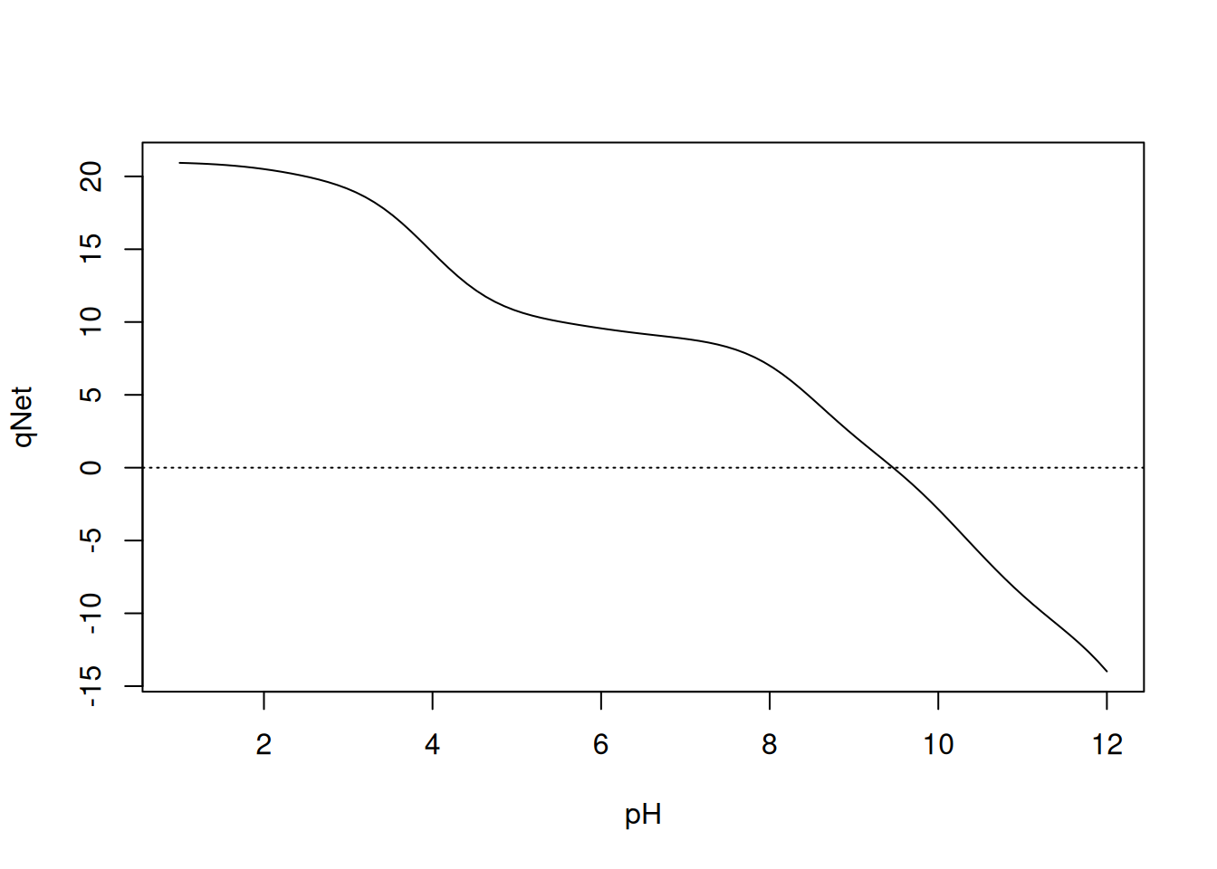
Note that the value found for pI of lysozyme was 9.46; that is, at pH 9.46 the enzyme presents a net net charge of zero, as can also be seen in the graphical representation.
Isoionic point & R libraries
Despite the precision of the pI calculation by the numerical solution performed for lysozyme, one of the most fascinating features of the program lies in the use of libraries (
Among the existing libraries for physicochemical properties of proteins and nucleic acids, the
packages), which is no different for determining biopolymer properties, such as pI.Among the existing libraries for physicochemical properties of proteins and nucleic acids, the
seqinr package, Biological Sequences Retrieval and Analysis 1, for exploratory analysis and visualization of biopolymers, is an example. To use this package, however, it is necessary to obtain the primary sequence of the protein, represented in a one-letter code. The primary sequence of lysozyme can be obtained from the website of the National Center for Biotechnology Information, NCBI 2. A quick trick involves:type the name of the protein;
select from the resulting options;
click on FASTA to obtain the 1-letter primary sequence.
copy the presented protein sequence to
seqinr.
Assuming that the
seqinr library is installed, and that the sequence has been obtained for lysozyme (search for CAA32175 or lysozyme [Homo sapiens]), the pI value for it can be found using the following code:library(seqinr)
lysozyme <- s2c("KVFERCELARTLKRLGMDGYRGISLANWMCLAKWESGYNTRATNYNAGDR
STDYGIFQINSRYWCNDGKTPGAVNACHLSCSALLQDNIADAVACAKRVV
RDPQGIRAWVAWRNRCQNRDVRQYVQGCGV")
# convert string sequence to character vector
computePI(lysozyme)[1] 9.2778Note that the pI value for the package, 9.28, was very close to that found by the numerical solution above. This is due to the use of different algorithms for both, as well as the computation of different pKa values for
seqinr. As an example of this variation, seqinr itself presents different pKa values, depending on the database searched. To verify this, type the command below and view the resulting pK variable.library(seqinr)
data(pK)Additionally, you can also compare the pI value of lysozyme with the algorithm used by the database on the 3 website. To do this, simply paste the residue sequence into the available field and click on the pI computation. Note that the resulting value of 9.28 matches that of the algorithm used by the R
seqinr package.library(knitr)
knitr::kable(pK, "pipe", caption = "Table of pKa values for amino acids
from various sources, extracted from the seqinr package.")| Bjellqvist | EMBOSS | Murray | Sillero | Solomon | Stryer | |
|---|---|---|---|---|---|---|
| C | 9.00 | 8.5 | 8.33 | 9.0 | 8.3 | 8.5 |
| D | 4.05 | 3.9 | 3.68 | 4.0 | 3.9 | 4.4 |
| E | 4.45 | 4.1 | 4.25 | 4.5 | 4.3 | 4.4 |
| H | 5.98 | 6.5 | 6.00 | 6.4 | 6.0 | 6.5 |
| K | 10.00 | 10.8 | 11.50 | 10.4 | 10.5 | 10.0 |
| R | 12.00 | 12.5 | 11.50 | 12.0 | 12.5 | 12.0 |
| Y | 10.00 | 10.1 | 10.07 | 10.0 | 10.1 | 10.0 |
There are other R packages that analyze amino acid and nucleotide sequences, including the calculation of pI, among which it is worth mentioning Peptides 4.