# Inputs:
L0, R0, and Kd
# Outputs:
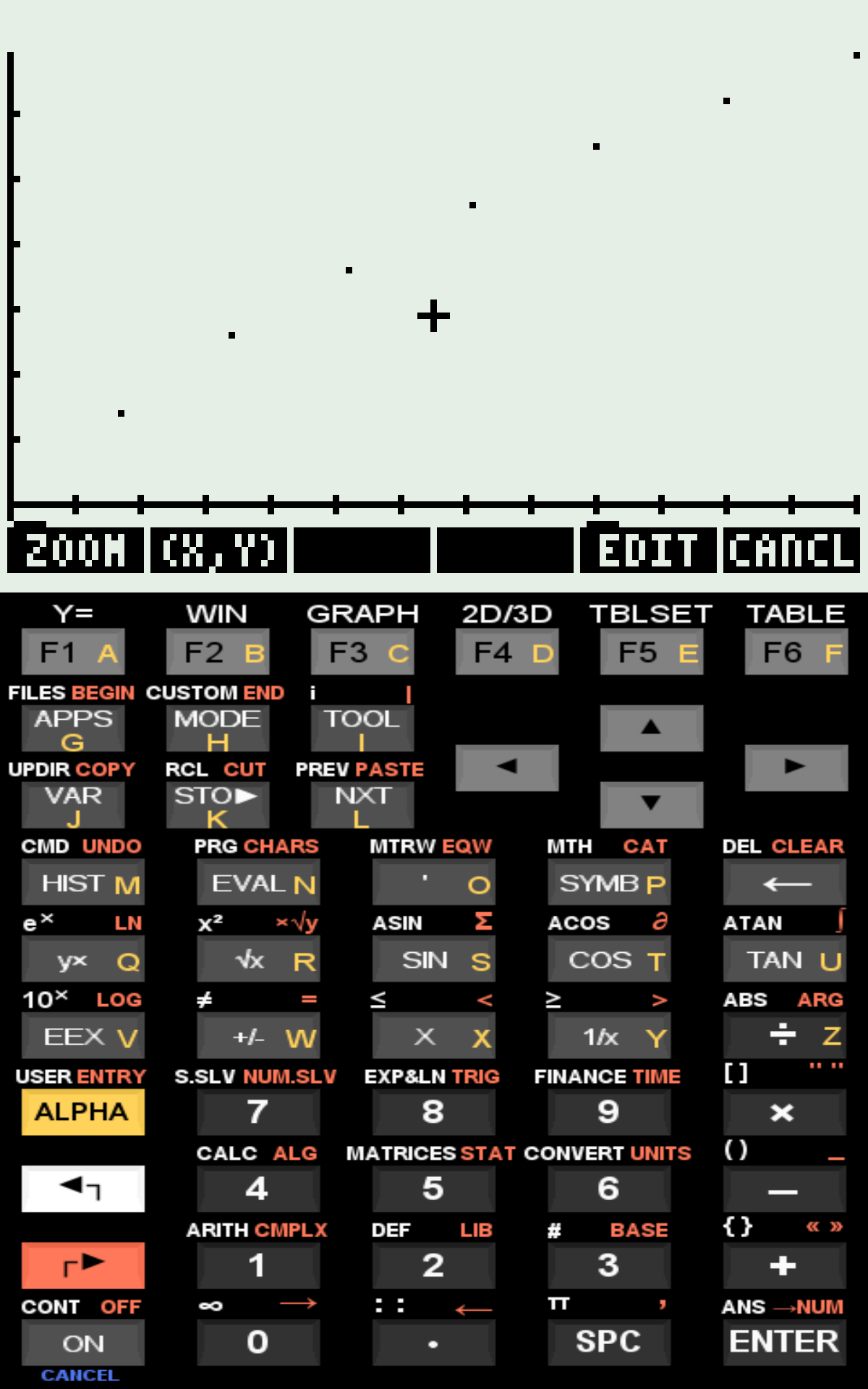
L × R plot;
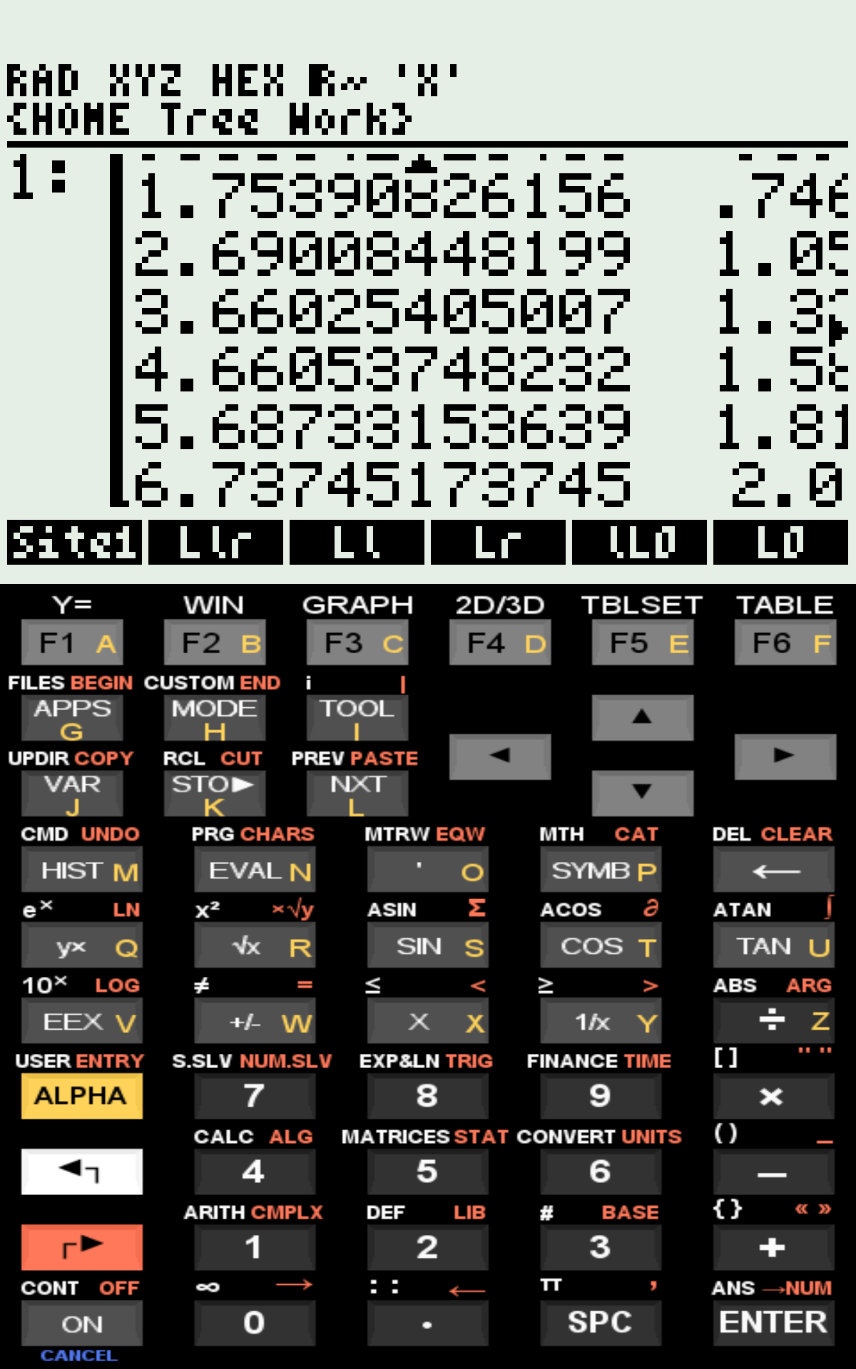
Matrix of L and LR values on the stack;
Variables (L, R, RL, initial values, and seeds).Numerical Solution for Interaction Equilibrium
There are generally two main approaches for solving mathematical problems in the Natural Sciences: analytical solutions and numerical solutions. An analytical solution (theoretical model) relies on a function containing one or more independent variables, a dependent variable, and one or more parameters to be determined, which together describe the problem situation. In contrast, a numerical solution does not depend on an explicit descriptive equation, but rather on approximations aimed at minimizing a general function (F(x) = 0). Numerical methods are employed when the theoretical model is complex, when an explicit solution is not desired, or when such a solution does not exist.
1 Equation:
The site1 program numerically solves the quantities involved in a bimolecular interaction equilibrium:
\[\begin{equation}
L + R \begin{array}{c}
_{k_{on}}\\
\rightleftharpoons\\
^{k_{off}}
\end{array} LR
\end{equation}\]
Where:
- R = free receptor (protein, nucleic acid, etc.);
- LR = formed complex;
- k\(_{on}\) = association rate constant of the complex;
- k\(_{off}\) = dissociation rate constant of the complex.
The equation describing complex formation is:
\[\begin{equation}
K_d = \frac{[RL]}{[R] + [L]} = \frac{k_{off}}{k_{on}}
\end{equation}\]
Where K\(_d\) represents the equilibrium dissociation constant of the complex. Thus:
\[ LR = \frac{L \cdot R}{K_d} \]
Accordingly, for the numerical solution of the theoretical model described above, the minimization functions are defined as:
\[ F(x)=0:\quad R_0 = R + LR ;;\rightarrow;; R + \frac{L \cdot R}{K_d} - R_0 = 0 \]
\[ F(x)=0:\quad L_0 = L + LR ;;\rightarrow;; \frac{L \cdot R}{K_d} - L_0 = 0 \]
2 site1
The program uses the MSLV (Multiple Equation Solver) command for the simultaneous solution of multiple equations, together with the MSLV2 library, which optimizes its performance. The library can also be loaded onto the calculator from its source code provided by the developer.
Program inputs and outputs are as follows:
3 Files:
4 Example of use:
1. Place on the stack:
  a. L0 = 10;
  b. R0 = 5;
  c. Kd = 10;

2. Run "Site1".
Although functional, the program is quite slow on HP50G hardware when compared to virtual versions or scientific desktop software. The example above takes about 16 seconds to complete the graph and output the variables, while the Octave program takes only 1 second.
References
- Olson, John S. Numerical analysis of kinetic ligand binding data. Methods in Enzymology, Vol. 76. Academic Press, 1981, pp. 652–667.