# Input:
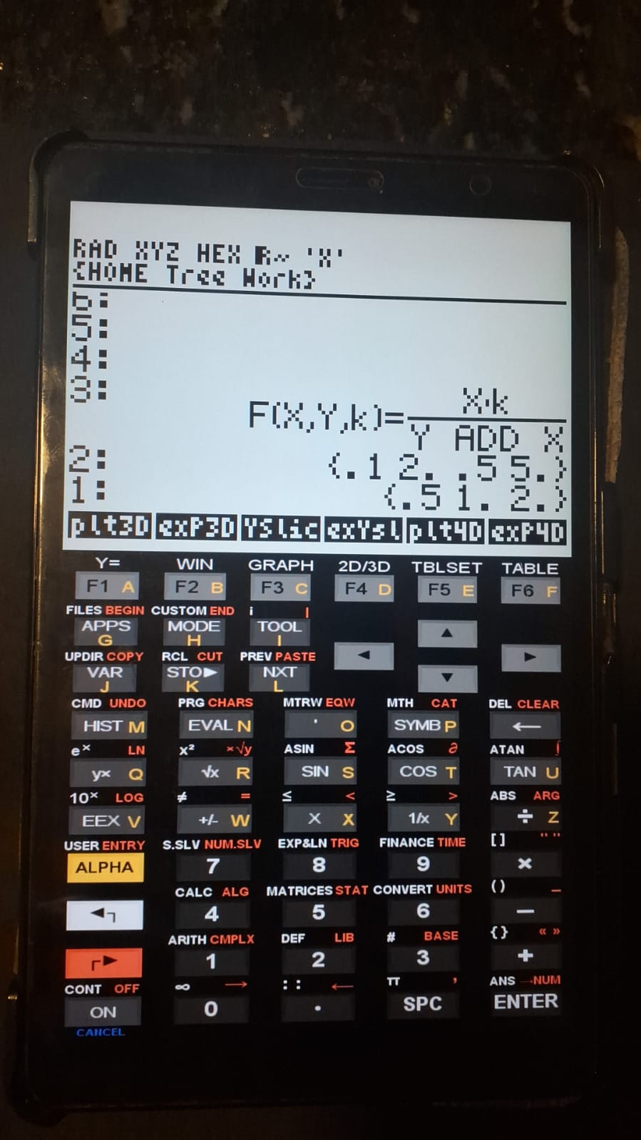
1. Formatted function; e.g., "F(X,Y,k) = (X*k)/(Y ADD X)";
2. List containing the limits of variables x and y; e.g., {0.1 2 0.5 5};
3. List of values for variation of parameter "k"; e.g., {0.5 1 2};
4. Run "SimPlot3D".
# Output:
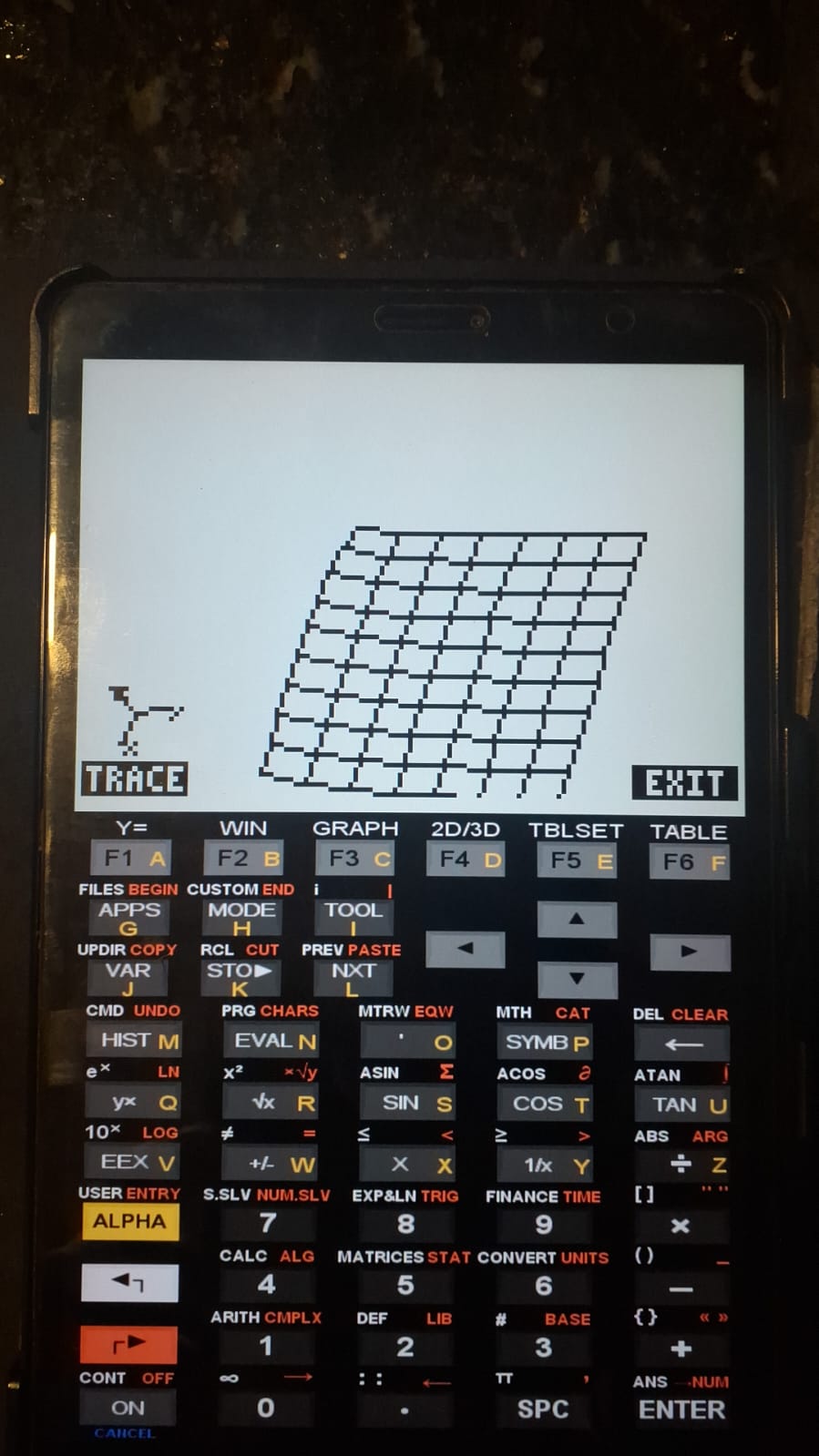
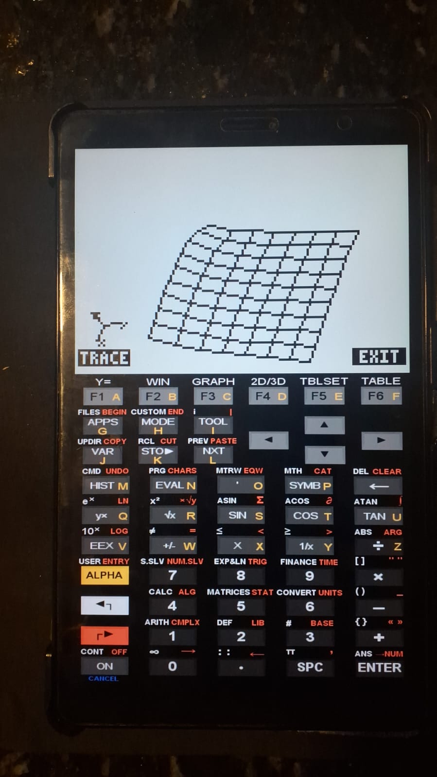
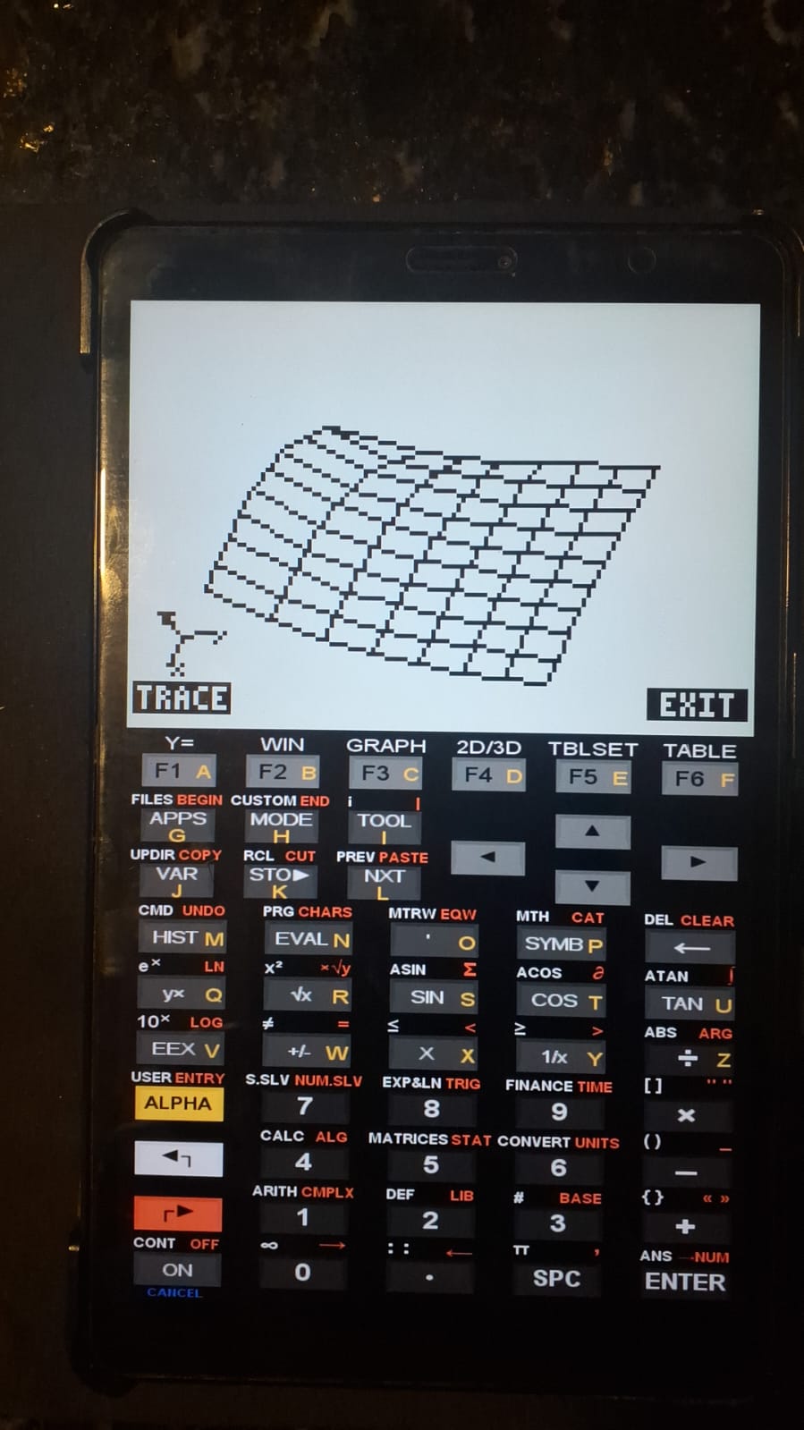
1. 3D wireframe plot for each value of "k"; switching between plots
is performed by pressing the EXIT key on the graphics screen;
2. Function and lists remaining on the stack for further modification.3D Simulation Plots with Parameter Variation
As with SimPlot, this program provides the same functionality, namely the visualization of the behavior of a graph as the value of a parameter (k) is varied. Unlike SimPlot, however, it offers three-dimensional wireframe visualization using the FAST3D command.
1 Equation
\[
z = f(x, y)
\]
For data input, the equation must be written in a specific format, as shown below:
\[ F(X,Y,k) = \text{function} \]
The function must explicitly include the parameter k and a list of its values. It should also be noted that, if the addition operation + is required, it must be written as ADD.
2 Files:
3 Usage and example
The figures below correspond to the example provided in the compressed file.