# Input:
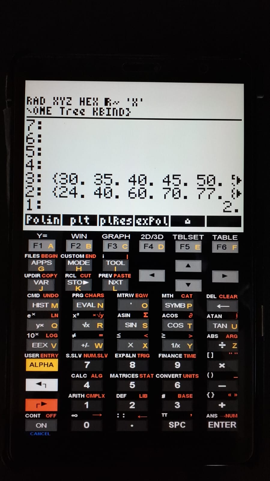
1. List of "x" values;
2. List of "y" values;
3. Polynomial degree.polFIT – Polynomial Regression and Gibbs–Helmholtz Curve as a Function of Temperature
Gibbs–Helmholtz curves, or stability curves as a function of temperature, are important in studies of folding, denaturation, and biomolecular interactions (Licata and Liu, 2011). Unlike the linear Van’t Hoff profile, they indicate changes in the heat capacity of the system and exhibit a curvilinear behavior that can be modeled using polynomial fitting.
The polFIT program performs polynomial regression using data provided as lists and a user-defined polynomial degree, presenting statistical fitting parameters as well as the scatter plot with the fitted curve superimposed.
1 Equation
Considering a general second-degree polynomial:
\[ y = a + b x + c x^2 \]
It is possible to approximate the thermodynamic quantities \(\Delta H\) (enthalpy), \(\Delta S\) (entropy), and \(\Delta C_p\) (heat capacity) that describe the phenomenon as a function of temperature using the relationships below (Waelbroeck and Van Obberghen, 1979):
\[ \Delta G = a + bT + cT^2 \]
\[ \Delta S = -\left(\frac{\partial \Delta G}{\partial T}\right)_p = -(b + 2cT) \]
\[ \Delta H = \left(\frac{\partial (\Delta G/T)}{\partial (1/T)}\right)_p = \Delta G + T \Delta S = a - cT^2 \]
\[
\Delta C_p = \left(\frac{\partial \Delta H}{\partial T}\right)_p = -2cT
\]
Thus, by solving for the polynomial coefficients, the thermodynamic quantities involved in the process can be obtained.
2 Files
3 Usage and example
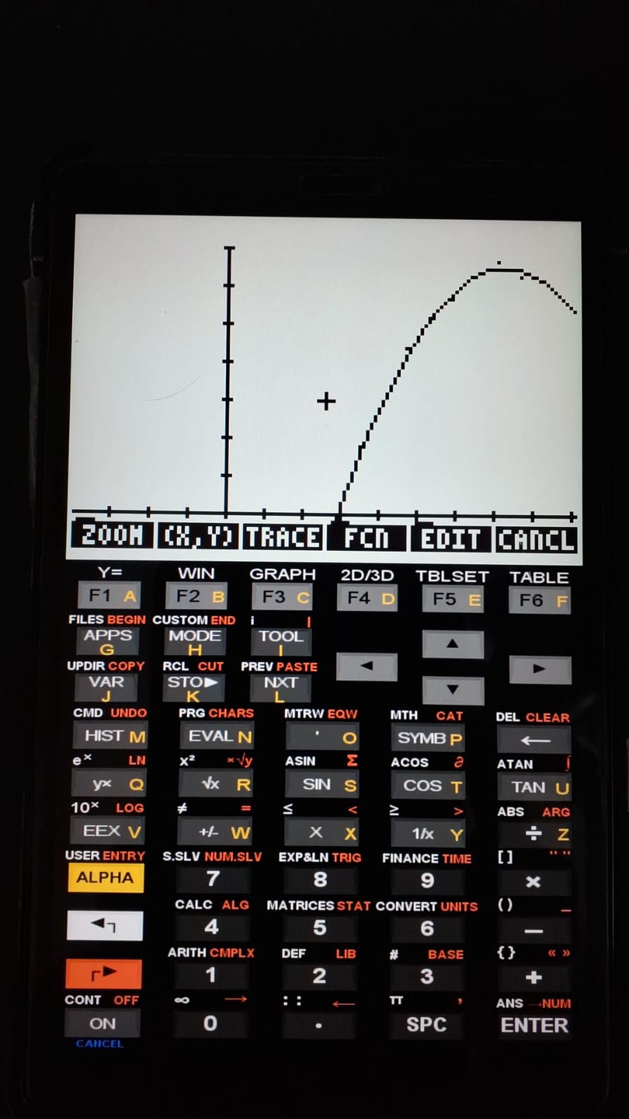
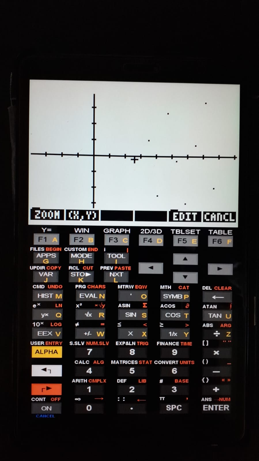
From a list of x values, a list of y values, and the polynomial degree, polFIT returns several fitting parameters. Two additional programs, polPlot and polRes, generate respectively the scatter plot with the fitted curve and the regression residual plot. The program requires the following data to be entered sequentially on the stack:
When running polFIT, the following outputs are generated:
# Output:

1. coef: polynomial coefficients;
2. se: standard errors of the coefficients;
3. qmreg: mean square of the regression;
4. sqres.sse: sum of squared errors (SSE);
5. qmres.s2: mean square of residuals;
6. sst: total sum of squares;
7. r2: coefficient of determination;
8. F: Snedecor’s F value;
9. pval: p-value of the regression.
The polynomial fitting of the example data yields the quantities and graphical profiles illustrated below.
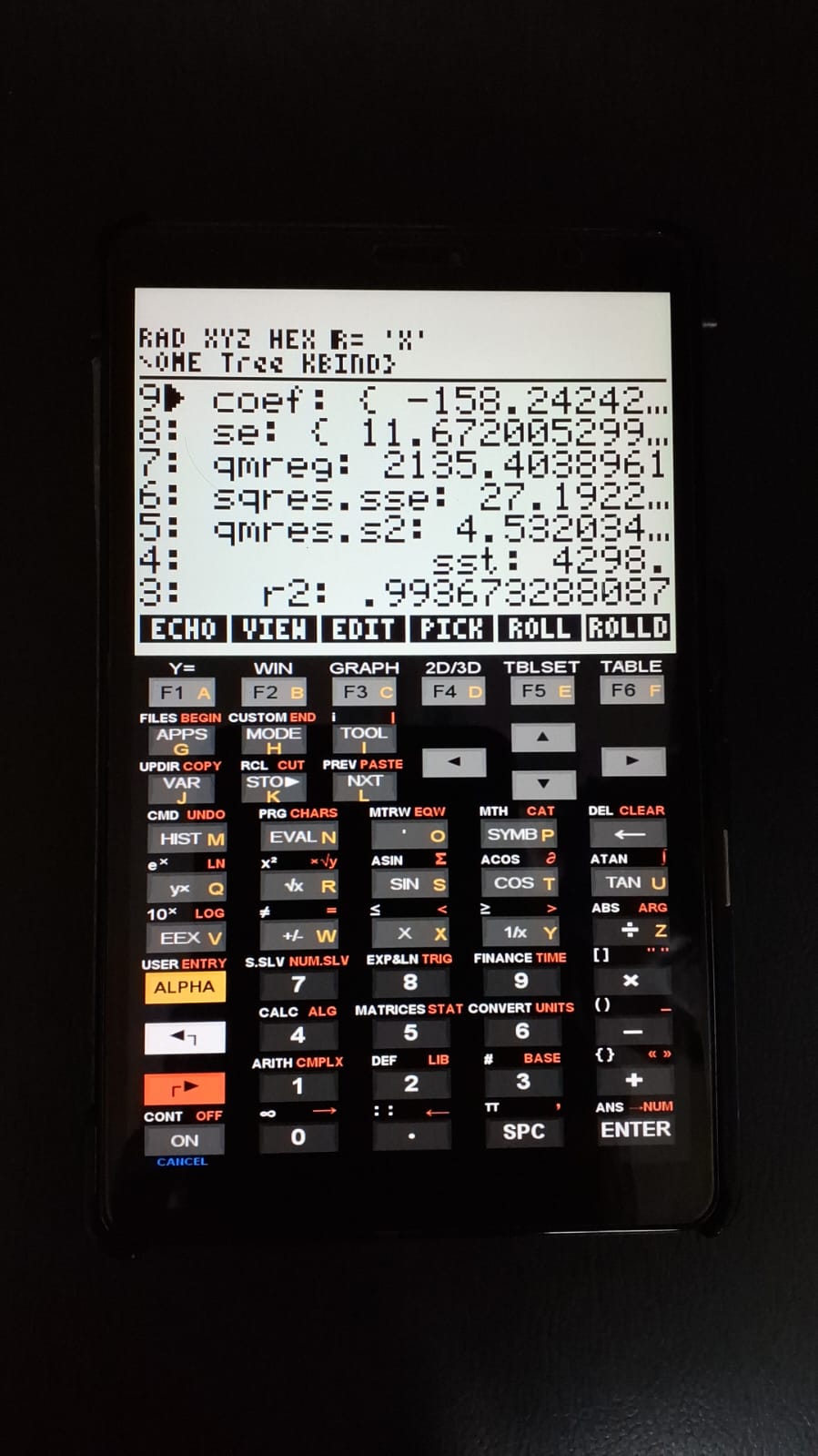
For the second-degree polynomial fit, the estimated coefficients were a = −158.24, b = 7.99, and c = −6.5 × 10\(^{-2}\). Substituting these values into the equations above, the thermodynamic quantities at 50 K are \(\Delta H\) = −20.1 kJ/mol, \(\Delta S\) = 1.5 J/mol/K, and \(\Delta C_p\) = 6.5 J/mol.
References
Licata, V. J., & Liu, C. C. (2011). Analysis of free energy versus temperature curves in protein folding and macromolecular interactions. In Methods in Enzymology (Vol. 488, pp. 219–238). Academic Press.
Waelbroeck, M., Van Obberghen, E., & De Meyts, P. (1979). Thermodynamics of the interaction of insulin with its receptor. Journal of Biological Chemistry, 254(16), 7736–7740.