nlFitNR - Nonlinear regression by Newton–Raphson and the Michaelis–Menten model

This program performs nonlinear least-squares regression for a user-defined equation. It uses an iterative procedure based on a first-order (truncated) Taylor expansion and solves for a parameter update vector that reduces the sum of squared residuals.

The Newton–Raphson algorithm implemented here follows these steps: (1) symbolic differentiation of the model with respect to each parameter, (2) numerical evaluation of these derivatives from user-provided seeds, (3) construction of the resulting Jacobian matrix of total derivatives, and (4) computation of the update \(\Delta a\) between the current parameter estimate and its seed, together with associated errors.

This program is similar to nlFIT hosted at hpcalc.org, but differs by: (1) using a different algorithm, (2) being ~30% shorter, (3) allowing one iteration at a time (useful given the slowness of RPL on physical hardware), (4) not including an automatic stopping criterion, (5) reporting parameters and their errors at each iteration, and (6) providing a separate plotting program to be run after the user decides that enough iterations have been performed. In short, it is a distinct algorithm and codebase, offering finer execution control. The implementation is based on the NLFIT algorithm adapted from Wickes (1992, p.666).

1 Equation

Using a first-order Taylor expansion around \(a_0\), the model can be linearized as:

\[ \phi(x,a)\approx\phi(x,a_0)+\sum_{j=1}^{p} \left.\frac{\partial \phi(x,a)}{\partial a_j}\right|_{a_0},\Delta a_j \]

Where:

\(\phi(x,a)\) = model (fitting) equation
\(a_j\) = model parameters
\(a_0\) = parameter seed (or the parameter vector at iteration \(i\))
\(\Delta a_j\) = parameter update for \(a_j\)

Defining the Jacobian entries as:

\[ X_{ij}= \left.\frac{\partial \phi(x_i,a)}{\partial a_j}\right|_{a_0} \]

the linearized least-squares step has the form:

\[ y \approx X,\Delta a \]

where \(X\) is the Jacobian matrix evaluated at \((x_i,a_0)\).

2 Files and example

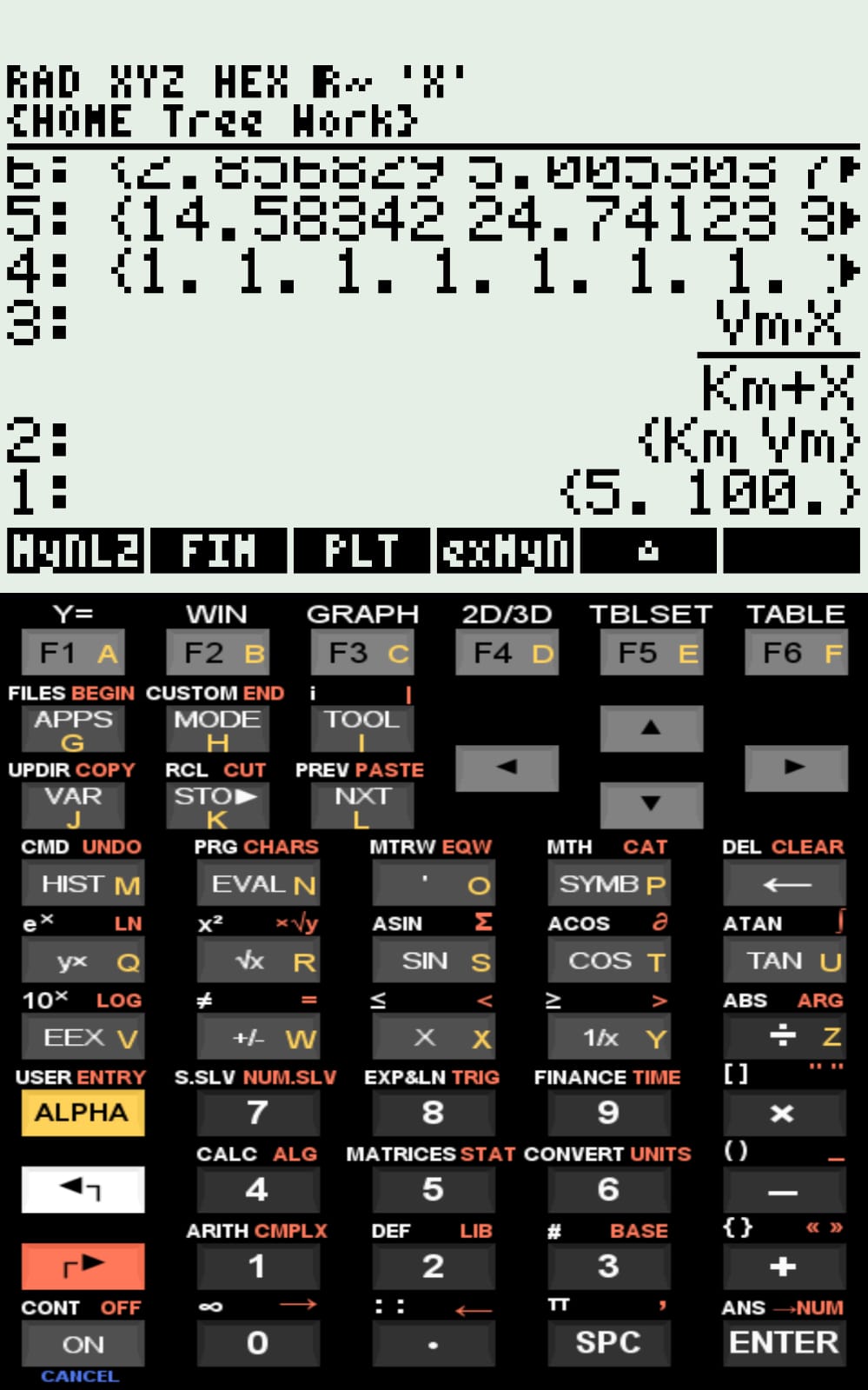
The program runs independently. The final plot (points plus fitted curve) is produced by a separate program (PLT). To use nlFitNR, the following items must be placed on the stack in order:

# Input data (stack order)

1. list of x_i values: {x1 x2 ... xn};
2. list of y_i values: {y1 y2 ... yn};
3. list of weights: {w1 w2 ... wn}.
   Note: if no weights are used, enter a unit list: {1 1 ... 1};
4. fitting function (e.g., Vm*x/(Km+x) for Michaelis–Menten).
   Note: use "x" as the independent variable;
5. list of parameters: {p1 p2}.
   In the example: p1 = Vm and p2 = Km;
6. list of parameter seeds.

The example data come from the L.minor dataset (nitrogen uptake by macrophytes), as presented in the nlstools package of the statistical software R.

# How to run

1. Press EVAL on the example file to unpack the input lists;
2. Run "nlFitNR";
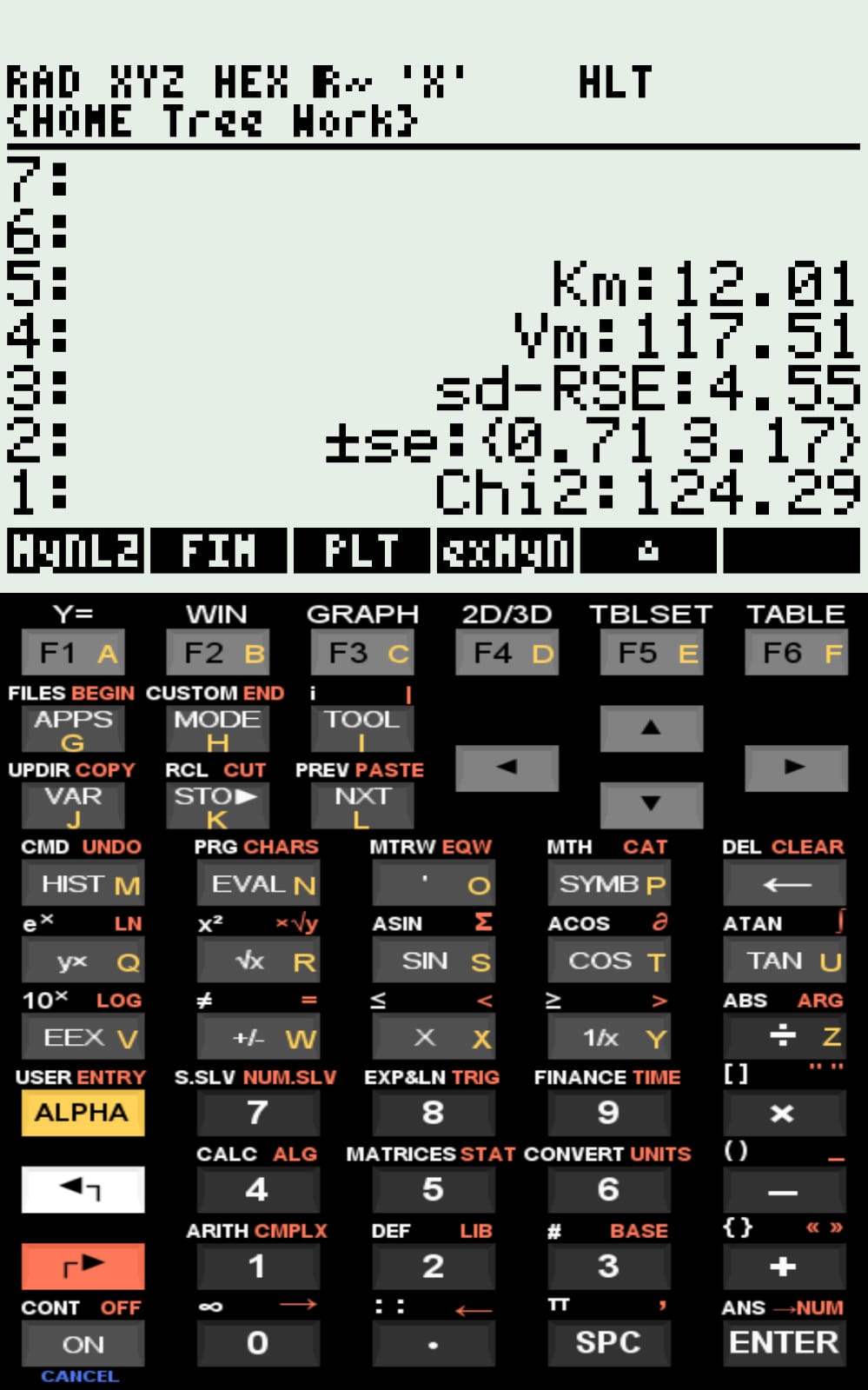
3. The program outputs:
   a. updated parameters (stack);
   b. "sd-RSE"  - residual variance of the fit;
   c. "+/- se"  - standard errors of the parameters;
   d. "Chi2"    - chi-square value of the fit;

4. If satisfied, interrupt the program (KILL) and inspect the plot.
   If not, run one more iteration by pressing "CONT".

Note: for your own data, simply replace the input lists.

3 Results

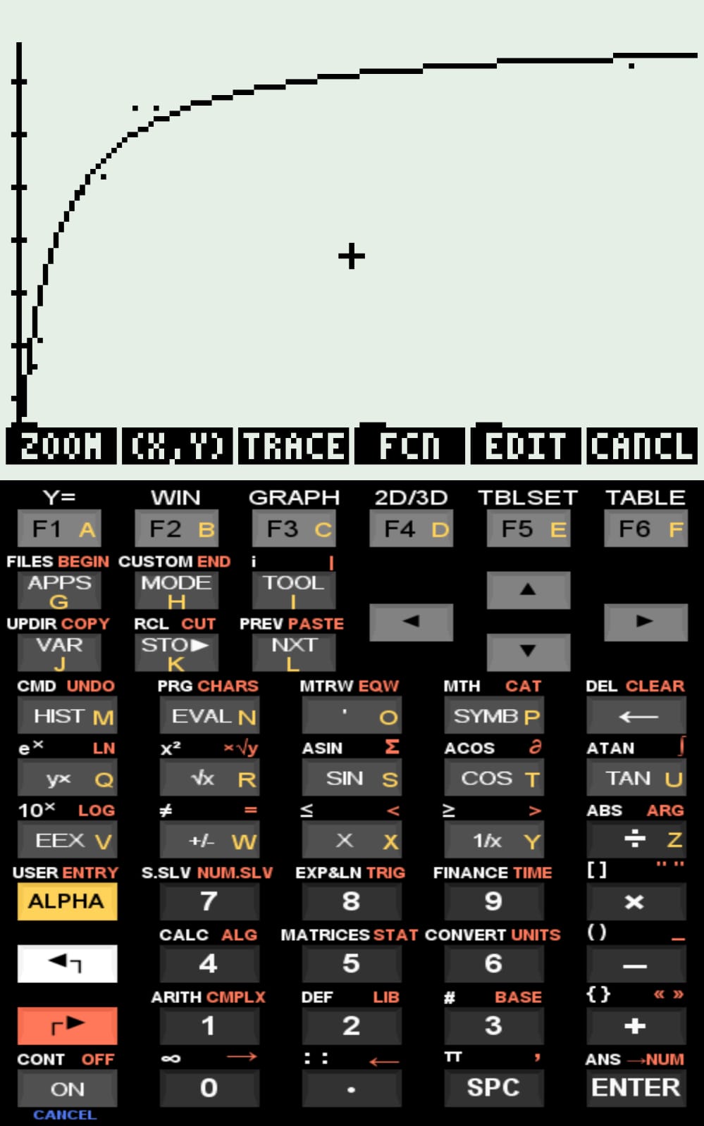
(a) Data entry. The bundled example requires EVAL to unpack the list.

The regression results approach those obtained with the statistical software R (table below) already in the first iteration, and the error metric (\(\chi^{2}\)) is reduced by about half. Subsequent iterations reduce the parameter uncertainties but may increase the global fit error. Values matching those obtained with R were reached by the third iteration.

Parameter	nlFitNR	R
Km	12.01 ± 0.71	17.079 ± 2.953
Vm	117.51 ± 3.17	126.033 ± 7.173
Iterations	1	7
\(\chi^{2}\)	124.29	234.375

References

Wickes, W.C. Hp 48 Insights. Part II: Problem Solving Resoruces (Hp 48G/Gx Edition), Larken Pub., 1992.