1. linFIT  - weighted linear regression;
2. Plt     - plot of the fit with regression line;
3. PlAdd   - overlay of plots on the display;
4. exLin - enzymatic inhibition example.Weighted Linear Regression and the Lineweaver–Burk Model
Linear fitting or regression is ubiquitous in the Sciences, among other reasons due to the statistical simplicity of the least-squares modeling involved (requiring only variations in sums of x, y, and x·y), the absence of iterative procedures or algorithms, and the possibility of understanding nonlinear models through linearization strategies. Nevertheless, such linear transformations also introduce statistical distortions, which may be corrected by incorporating weights into the fitting procedure.
Accordingly, weighted linear regression is particularly useful in situations involving error dispersion arising from linearization, as well as heteroscedasticity. Below, three HP50 programs are presented for weighted linear fitting and graphical visualization, together with a test example:
1 LinFIT
The linFIT program employs linear algebra to determine the coefficients a and b of a weighted linear fit, together with additional statistical parameters such as standard errors of the parameters, covariance, and sum of squared errors (SSE), among others.
2 Equation:
\[ y = a + b,x \]
\[ \beta = (X^{T} w X)^{-1} X^{T} w y \]
Where:
- \(\beta\) = matrix of coefficients (a and b);
- X = matrix of x values with a unitary first column;
- \(X^{T}\) = transpose of X;
- y = matrix of y values;
- w = weight matrix.
3 Files:
To use the plotting programs, simply unzip the file and place the programs in a calculator directory, such as HOME.
4 Example of use:
The file includes the programs and an example of Lineweaver–Burk linearization applied to enzymatic inhibition (Cornish-Bowden, 2014), using data from Wilkinson (1961). The file “exLin” contains the required data for the program in the form of a list. The list consists of the x and y variables, as well as a unitary weight w (see figure below).
Lists are particularly well suited for the HP50, since when working in RPN and stack-based operations, a list can be rapidly transformed through arithmetic operations without the need for commands typically required for other data structures such as vectors or matrices, as illustrated below.
1. Place the file "exLin" on the stack and press EVAL, resulting in three lists (x, y, and w);
2. If no weighting is required, simply run "linFIT" to obtain the parameters, in the following order:
covXY (covariance), s2x (variance in x), s2y (variance in y),
s2 (variance of the fit), F (Snedecor’s F value),
intcp (intercept), se (standard error of the intercept),
slope (slope), se (standard error of the slope),
ChiSQ (chi-square value), and pval (p-value of the fit);
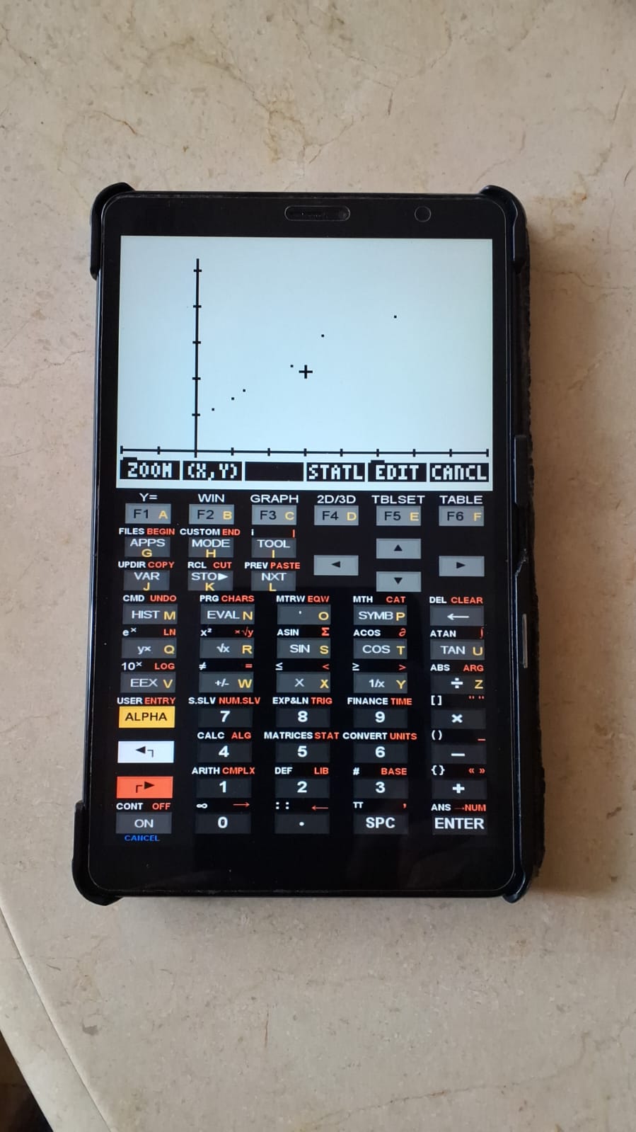
3. Run "Plt" to visualize the plot;
4. In the graphical area, select STATL to display the regression line.
# Use of weights in the fitting
1. Place "exLin" on the display and press EVAL;
2. Remove the unitary weight list (DROP or back arrow);
3. Obtain a weight of 1/v²:
a. Press ENTER to duplicate the *y* list;
b. Apply x² to square the list;
c. Apply 1/x to obtain the reciprocal of the squared *y* values;
4. Run "linFIT".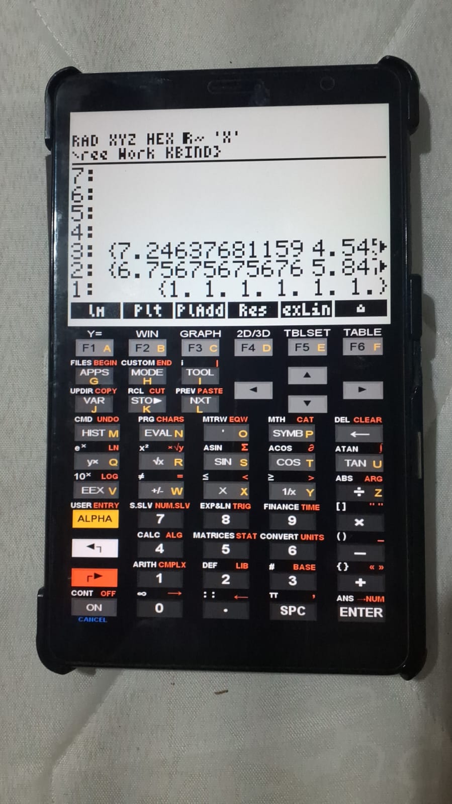
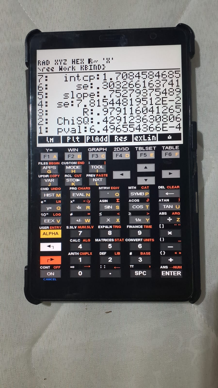
To compare fits obtained with different weighting schemes, simply select “PlAdd” from the auxiliary program (for the example provided, differences are minimal). The estimated values for the slope (Km/Vm; 0.80 ± 0.07) and intercept (1/Vm; 1.54 ± 0.15) are consistent with those reported by Wilkinson (1961), using a weight of 1/v\(^{2}\).
References
- Cornish-Bowden, A. Analysis and interpretation of enzyme kinetic data. Perspectives in Science, 1(1–6), 121–125, 2014.
- Wilkinson, G. N. Statistical estimations in enzyme kinetics. Biochemical Journal, 80(2), 324, 1961.