# Inputs
k1 = 0.02;
k2 = 0.001;
tol = 1e-5 (tolerance);
x = 0 (initial time);
y = [0.8 1 0] (initial vector for L, R, and LR);
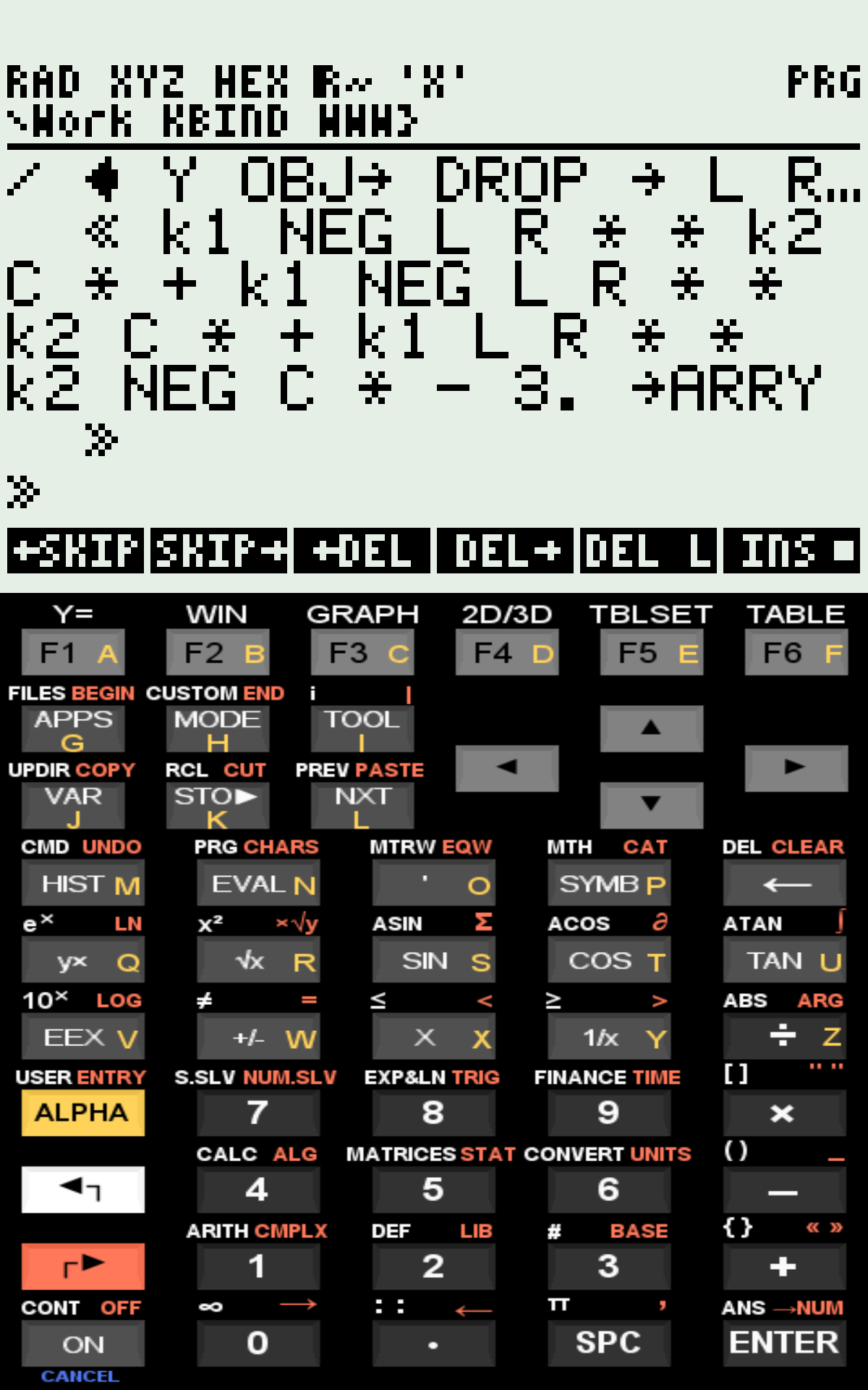
F (RPN subroutine for the 3 equations)
Run "kinSite"
# Outputs
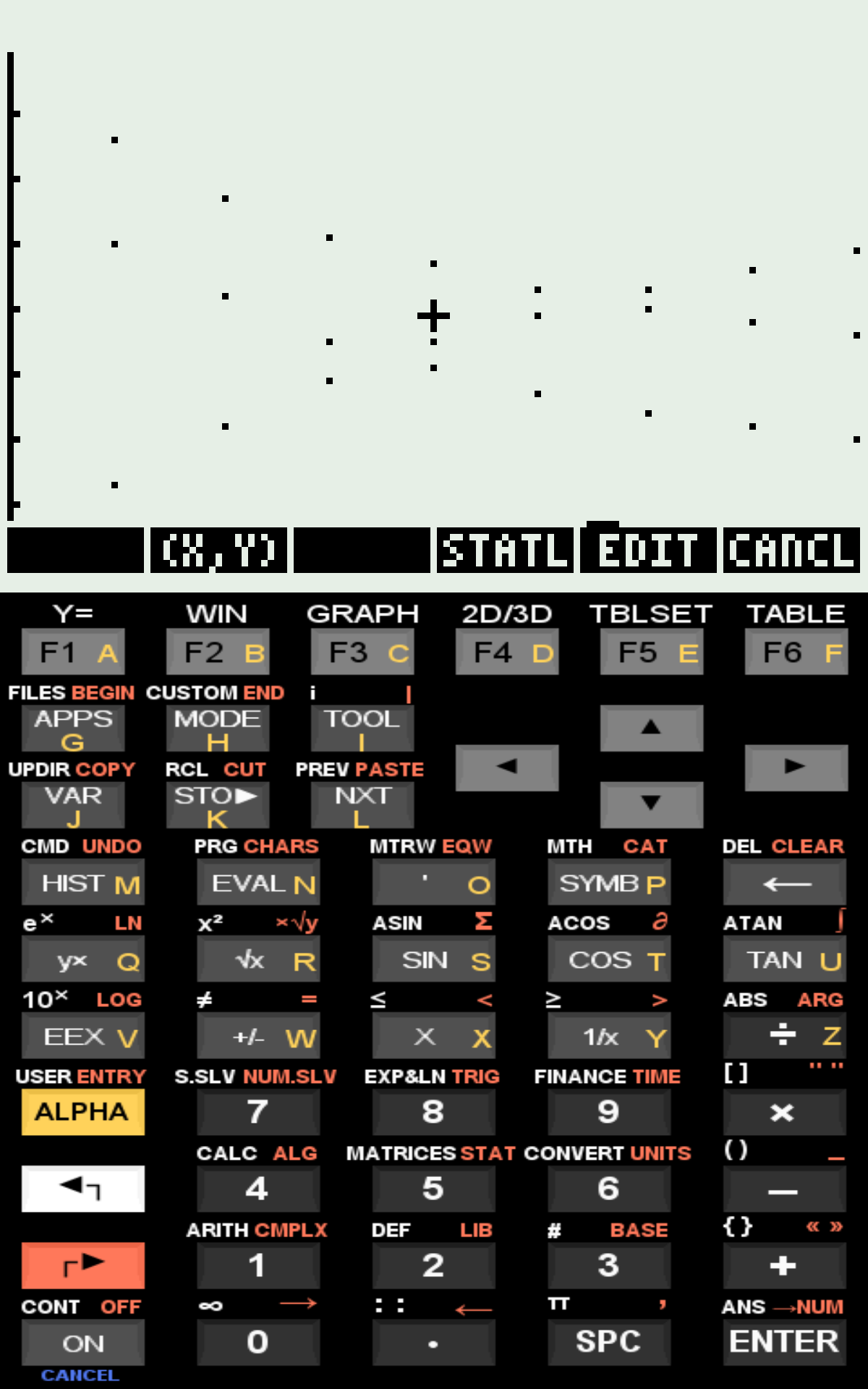
Plot of t vs. L, R, and LR;
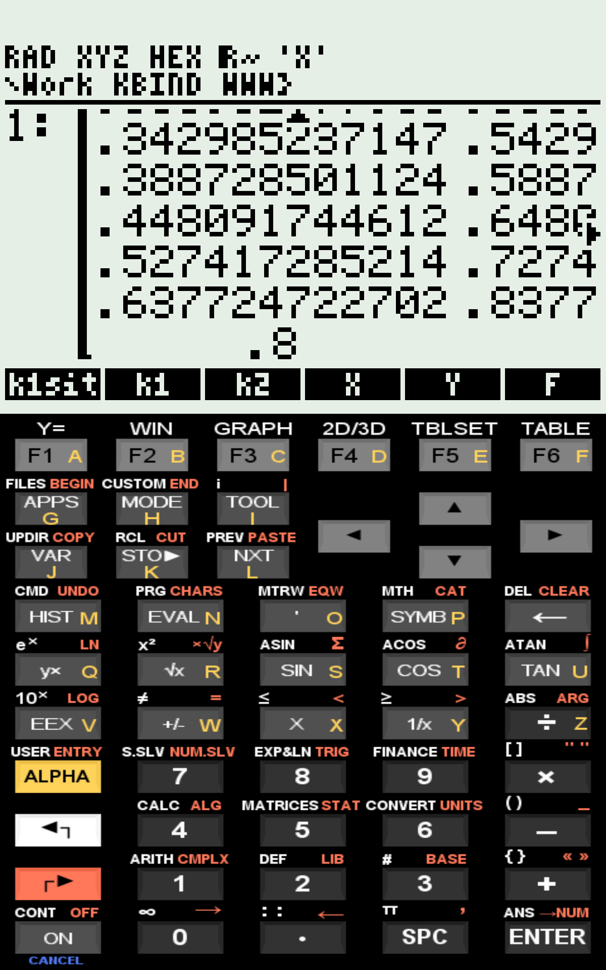
Matrix of computed values on the stack;Ordinary Differential Equations (ODEs) and Ligand–Receptor Binding Kinetics
In parallel with the numerical solution of multiple equations (program Site1), a broad range of scientific problems involves rates of change of one or more quantities with respect to one or more independent variables—situations naturally described by differential equations. When a single independent variable is involved (typically time), these derivatives are referred to as ordinary differential equations (ODEs). Solving an initial value problem for an ODE is commonly done through numerical approximation schemes, among which the classical fourth-order Runge–Kutta–Fehlberg method is widely known. The kinSite program uses the calculator’s internal ODE solver (RKF) to model the kinetics of molecular interaction.
1 Equation
The interaction considered here is a bimolecular ligand–receptor reaction:
\[\begin{equation}
L+R \begin{array}{c}
_{k_1}\\
\rightleftharpoons\\
^{k_2} \end{array} LR
\end{equation}\]
Where:
- R = free receptor (protein, nucleic acid, etc.);
- LR = complex formed;
- k\(_1\) = association rate constant;
- k\(_2\) = dissociation rate constant.
The association rates are described by:
\[ \frac{d[LR]}{dt}=k_1[L][R] \]
\[ \frac{d[L]}{dt}=-k_1[L][R] \]
\[ \frac{d[R]}{dt}=-k_1[L][R] \]
Likewise, the dissociation rates are given by:
\[ \frac{d[LR]}{dt}=-k_2[LR] \]
\[ \frac{d[L]}{dt}=k_2[LR] \]
\[ \frac{d[R]}{dt}=k_2[LR] \]
At equilibrium (and, more generally, along the full time course), the net reaction rates are the sum of association and dissociation contributions. Therefore, the system to be solved is:
\[ \frac{d[L]}{dt}=-k_1[L][R]+k_2[LR] \]
\[ \frac{d[R]}{dt}=-k_1[L][R]+k_2[LR] \]
\[ \frac{d[LR]}{dt}=k_1[L][R]-k_2[LR] \]
Numerically, the evolution of ([L]), ([R]), and ([LR]) over small time steps (t) can be computed from a system of differential equations in vector form:
\[ \Delta x=f(x),\Delta t \]
2 kinSite
The program uses the HP50G RKF routine (Runge–Kutta–Fehlberg) to solve the ODE system numerically. The algorithm computes ([L]), ([R]), and ([LR]) along time and plots the resulting kinetic curves. Data entry requires a subroutine containing the ODE system written in postfix (RPN) syntax (figure).
Example inputs and outputs are:
3 Files
As with Site1, kinSite is relatively slow on the physical calculator (~30 s), although it runs essentially instantaneously in virtual versions or scientific suites. Nearly identical results were obtained in ~1 s using the approach described by Prinz (2011, ch. 6) with Octave (function lsode).
References
- Prinz, Heino. Numerical Methods for the Life Scientist: Binding and Enzyme Kinetics Calculated with GNU Octave and MATLAB. Springer Science & Business Media, 2011.