# Inputs
k1 = 1000;
km1 = 0.1;
k2 = 0.05;
E0 = 0.005;
tol = 1e-5 (tolerance);
x = 0 (initial time);
y = [0.001 0 0] (initial vector for S, ES and P)
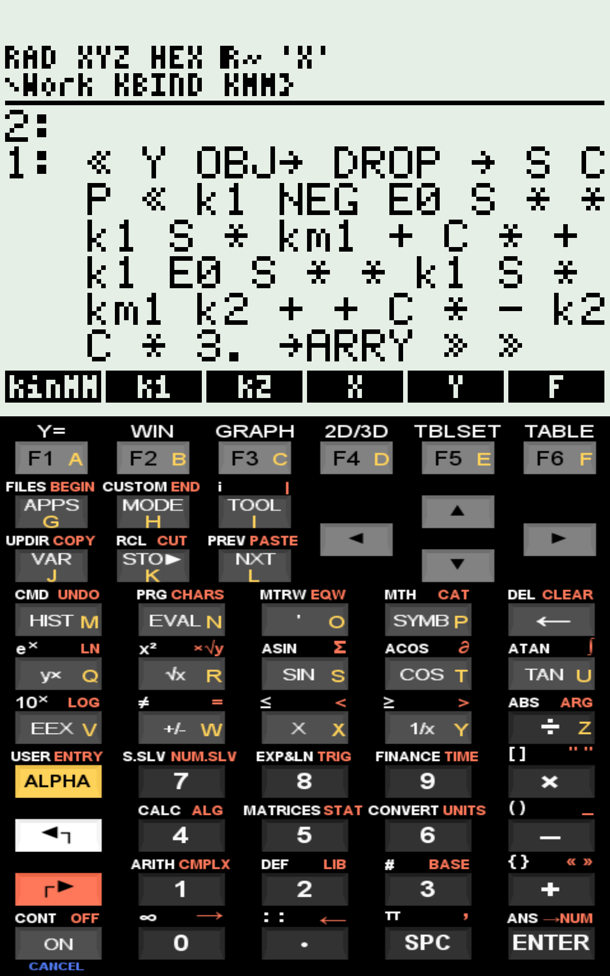
F - RPN subroutine defining the 3 equations
Run "kinMM"
# Outputs:
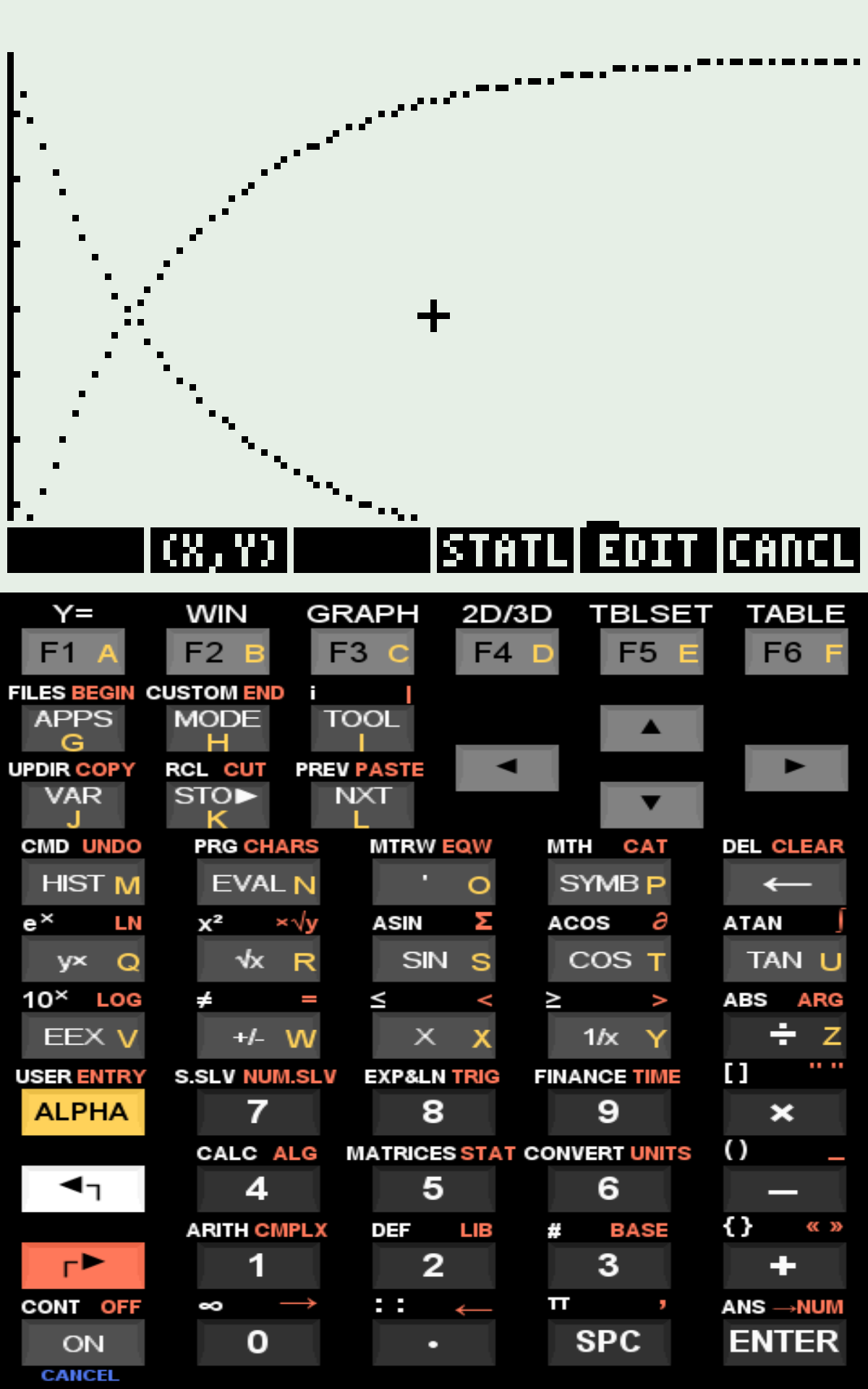
Plot of t vs S and P;
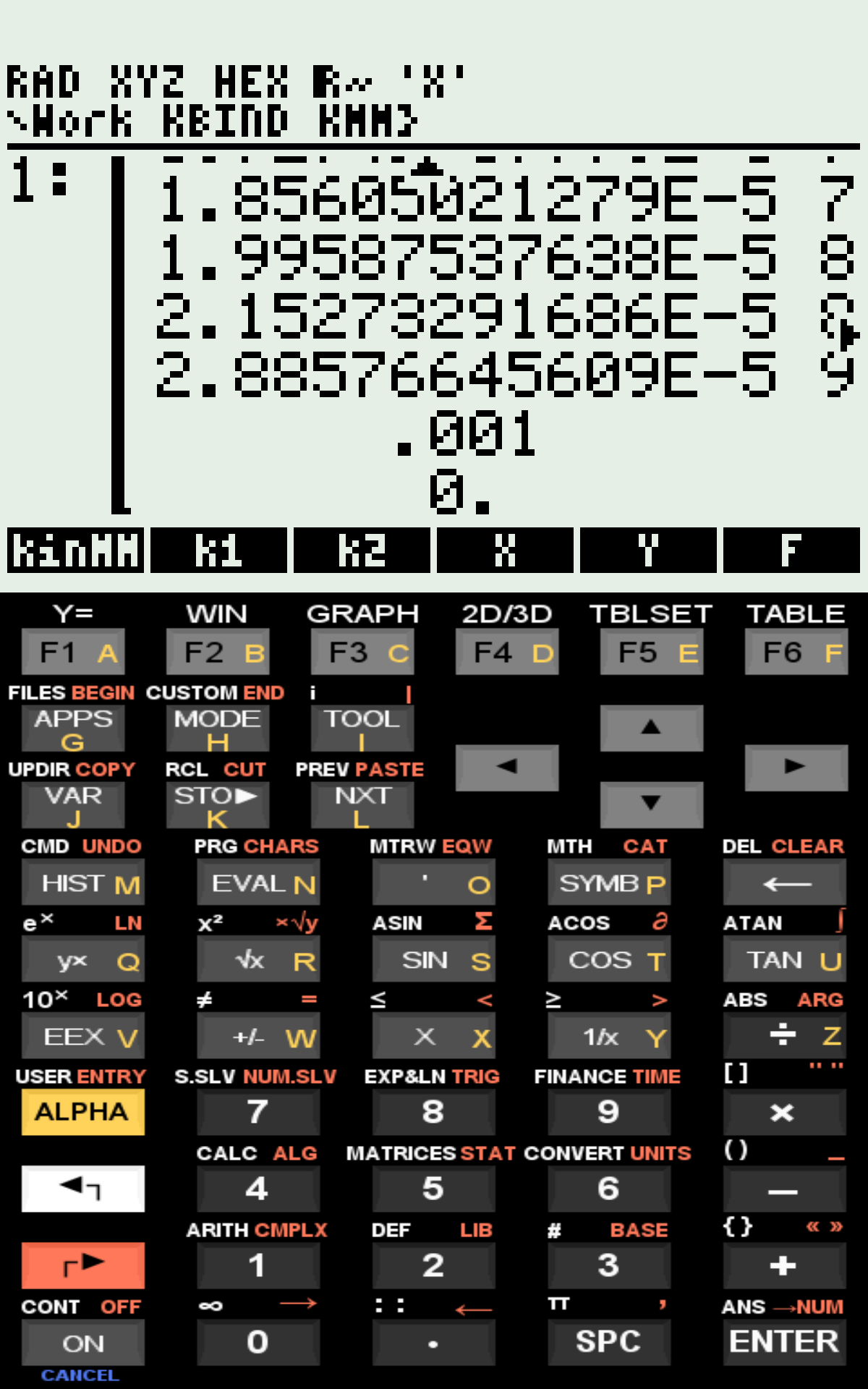
Matrix containing S, ES, P and t values on the stack;Ordinary Differential Equations (ODE) and Michaelis–Menten Kinetics
As previously applied to binding kinetics in the kinSite program, the fourth-order Runge–Kutta–Fehlberg method can also be employed to solve other ordinary differential equations (ODEs), such as those describing Michaelis–Menten enzyme kinetics.
The program kinMM implements the numerical solution of an initial value problem using the RKF command available in the HP50G calculator.
The program kinMM implements the numerical solution of an initial value problem using the RKF command available in the HP50G calculator.
1 Equation
The program kinMM solves the time evolution of S (substrate), E (enzyme), ES (enzyme–substrate complex), and P (product) according to the classical catalytic scheme:
\[ E + S ;\underset{k_{-1}}{\stackrel{k_{1}}{\rightleftharpoons}}; ES ;\xrightarrow{k_{2}}; E + P \]
Where:
- S = substrate
- E = free enzyme
- ES = enzyme–substrate complex
- P = product
- \(k_{1}\) = association rate constant
- \(k_{-1}\) = dissociation rate constant
- \(k_{2}\) = catalytic rate constant
The kinetic behavior of the system is described by the following system of ordinary differential equations:
\[ \frac{d[S]}{dt} = -k_1 [E][S] + k_{-1}[ES] \]
\[ \frac{d[ES]}{dt} = k_1 [E][S] - (k_{-1} + k_2)[ES] \]
\[ \frac{d[P]}{dt} = k_2 [ES] \]
Since enzyme is conserved during catalysis:
\[ [E]_0 = [E] + [ES] \]
As in the kinSite binding model, the numerical solution is obtained by integrating the system:
\[ \frac{d\mathbf{x}}{dt} = f(\mathbf{x}) \]
or, in discrete approximation,
\[ \Delta \mathbf{x} = f(\mathbf{x})\Delta t \]
2 kinMM
The program uses the RKF function of the HP50G to compute the Runge–Kutta–Fehlberg numerical solution. The algorithm calculates the time evolution of S, ES, and P, and plots the kinetic profile showing substrate depletion and product formation.
Data input requires a subroutine written in postfix (RPN) syntax defining the system of differential equations (see figure).
Data input requires a subroutine written in postfix (RPN) syntax defining the system of differential equations (see figure).
Example of input and output:
3 Files
As with Site1 and kinSite, execution on the physical calculator is relatively slow (~20 s for 9 time points), whereas it is nearly instantaneous in virtual HP50G versions or scientific computing environments (e.g., Octave using custom scripts).
References
- Murray, J. D. Mathematical Biology II: Spatial Models and Biomedical Applications. Springer, 2003.