More interactivity!

Objectives:
1. Observe the extensive interaction capabilities of the “plotly” package
2. Create a graph with a slider
3. Create a graph with a drop-down menu

So far, we have only “scratched the surface” of the graphical interactivity potential of the plotly package. As already mentioned, this library allows for a wide range of user actions, such as sliders, drop-down menus, and buttons, among many others.

1 Adding a range slider

A slider of this nature allows you to choose a data window for a more detailed study in that region. In this case, it is possible to add a range slider to a simple graph.

We can illustrate its use by observing greenhouse gases, and in particular, carbon dioxide emissions in Brazil from an internet database. To do this, you will learn how to obtain a file from an internet database, filter it to a desired subset, and draw the resulting graph with an additional slider.

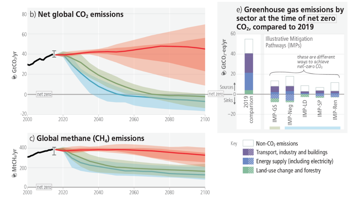
1.1 CO\(_{2}\) emissions and the greenhouse effect

Emissions of CO\(_{2}\) and other gases from the burning of fossil fuels are largely responsible for the greenhouse effect, directly affecting climate change. To reduce these emissions, it is necessary to transform the current energy matrix, industry, and food systems.

To understand CO\(_{2}\) emissions in Brazil from 1890 to 2022, run the following code snippet in an R script (i.e., copy, paste, and run) from the source Our World in Data.

library(readr) # data import library
library(dplyr) # library for using the pipe operator "%>%"
library(plotly)

# Loading data from the internet
url <- "https://raw.githubusercontent.com/owid/co2-data/master/owid-co2-data.csv"
co2_data <- read.csv(url)

# Filtering data for Brazil using subset()
co2_brasil <- subset(co2_data, country == "Brazil")

# Creating an interactive graph with plot_ly
co2_plot <- plot_ly(data = co2_brasil, x = ~year, y = ~co2, type = 'scatter', mode = 'lines+markers') %>%
layout(title = "CO2 emissions in Brazil over the years",
xaxis = list(title = "Year"),
yaxis = list(title = "CO2 emissions (million tons)"))

Now, the icing on the cake. The insertion of a slider to select ranges for a more focused study.

co2_plot %>%
rangeslider()

You can copy and paste the scripts in sequence for execution, or just add the command rangeslider() with the pipe operator %>% at the end.

Now try positioning the mouse on one of the two side markers of the lower graph, dragging it, and observe the result. The slider can be useful when you want to focus on a specific region of the graph. For example, to adjust CO₂ emissions for the last few years.

1.1.1 Adding a drop-down menu

Dropdown menus allow you to view a different graph for each option selected. To illustrate this interactive feature, let’s first create a dataset that has linear, quadratic, and cubic responses to an independent variable, as follows:

x = 1:10 # vector of the independent variable "x"
yLin = x
yQuad = x^2 # creation of the quadratic dependent variable 
yCub = x^3 # creation of the cubic dependent variable 

datLQC <-data.frame(x,yLin,yQuad,yCub) # creation of the data sheet

Now we can insert the dropdown menu for selecting mathematical trends:

plot_ly(datLQC, x = ~x, y = ~yLin, type = "scatter", mode = "line", name = "Linear") %>%
  add_trace(x = ~x, y = ~yQuad, mode = "line", name = "Quadrático") %>%
  add_trace(x = ~x, y = ~yCub, mode = "line", name = "Cúbico") %>%
  layout(
    title = "Gráficos de potência",
    xaxis = list(title = "x"),
    yaxis = list(title = "x^n"),
    updatemenus = list(
      list(
        buttons = list(
          list(label = "yLin", method = "update", args = list(list(visible = c(TRUE, FALSE, FALSE)))),
          list(label = "yQuad", method = "update", args = list(list(visible = c(FALSE, TRUE, FALSE)))),
          list(label = "yCub", method = "update", args = list(list(visible = c(FALSE, FALSE, TRUE))))
        )
      )
    )
  )

Although you may find the code snippet above a little complicated, just copy it, paste it into a script, and run it. This exemplifies the essence inherent in Reproducible Teaching, from the simple reproduction of code to its alteration and even the creation of new code. If you are curious, you can change some terms in the code above, such as the labels (label, replace a name, for example) that appear in the drop-down menu, the type of graph you want (replace scatter with bar, for example), or the title of the graph (title).

In terms of interactivity, the selection of the type of power to be represented by the drop-down menu is added to those already present in the plot_ly command.

As with many R packages, there are a significant number of commands and interactive widgets with plotly, which, in this specific case, would provide enough material for a separate book. However, you can consult numerous websites about plotly for more comprehensive learning, the links below, and even a free online book with related codes and graphics. To see the immense wealth of interactive graphics, take a look at the plotly website (https://plotly.com/r/) for R.

• General
• Manual
• Tutorial